Time is a circle (3/4)

This is the third post in a sequence following tardily on the heels of (1/4) and (2/4). Those give some impressionistic context while this will go right into methods and results.

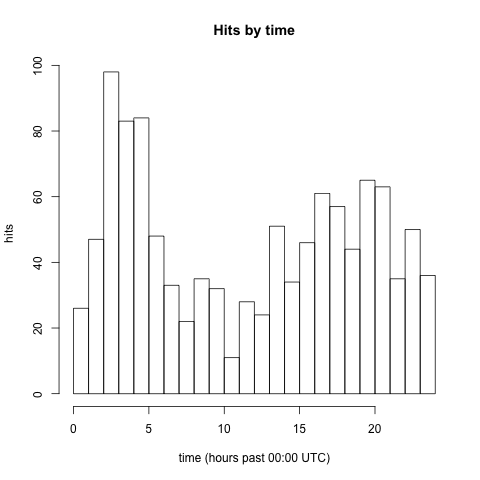
Histogram of (non-bot) website activity by time of day, showing data up to 2015-04-12.

Access time data can be thought to take values in the range [00:00 UTC, 24:00 UTC). I could try to justify treating this as a circular distribution just on the basis of the data but the most compelling comes from jumping ahead to the modeling stage. I want a model that:

1. treats times like 23:59 UTC as being similar to times like 00:01 UTC,
2. has a few parameters as possible (at least as a first step in analysis), and
3. is in the exponential family.

These considerations point to the von Mises distribution.

There are two complementary perspectives we can take on circular distributions. The more obvious one is to say that they describe angles.¹ Alternatively, we can say the distributions describe positions on the circle, in Cartesian coordinates or more elegantly as a complex number. We can go between the two using Euler’s identity \(z = e^{i x}\), where \(x\) is the angle in radians and \(z\) is the complex representation of a point on the circle.

(Exercise to the reader: does it make more sense to take the average of angles or of positions?

The von Mises distribution for the angle \(x\) (in radians) has probability density function \[f(x ; \mu, \kappa) = (2 \pi I_0(\kappa))^{-1} e^{\kappa \cos(x - \mu)}\] over the interval \([0,2\pi]\). Its location is set by \(\mu \in \mathbb{R}\) and its concentration (reciprocal of its “variance”²) set by \(\kappa > 0\). The term \(I_0(\kappa)\)³ is just a normalization constant, whose value ensures that the density integrates to \(1\). If you find the \(z\) perspective helpful, see footnote “⁴”.

Here are some properties of the von Mises distribution that are helpful in building intuition but can be safely skipped:

• In the large \(\kappa\) limit, the density is increasingly well-approximated by \(\text{Normal}(\mu, 1 / \kappa)\).
• (Exercise to the reader: what about the small \(\kappa\) limit?)
• (Exercise to the reader: why doesn’t/shouldn’t the normalizing constant depend on \(\mu\)?)
• (Exercise to the reader: if it’s in the exponential family, what are its sufficient statistics and natural parameters? Hint: apply trig identities to the cosine. Answer: see this passage.)
• Since the von Mises distribution is in the exponential family, its moments have fairly simple formulae and MLE inference proceeds by equating the expected moments with the observed ones.⁵ I defer to the circular R package to have worked out and implemented all the details.

So what happens when I fit this model to the access time data? The result is the opaque pair of numbers \(\mu_{rad}^* = -0.06\) and \(\kappa^* = 0.29\). If I convert back to time, this gives \(\mu^* = \text{23:47 UTC}\) and leaves \(\kappa^*\) unchanged. If more numbers are needed, I can also report the uncertainty in the estimates by giving the standard errors and say that \(\mu^* = \text{23:47UTC (9.0 minutes)}\) and \(\kappa^* = \text{0.29 (0.04)}\). I found creating some visualizations helpful in gaining more understanding of what the model says about the data.

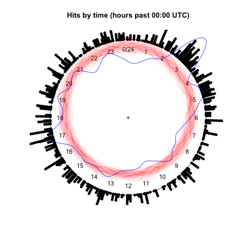
Visualization of maximum likelihood fit of von Mises distribution to time of day data.

There’s a lot going on here. The first thing to look at are the towers of black dots around the edge of the circle. Each dot is the time of an particular hit; this is just the histogram at the beginning, wrapped around the circumference of the circle so that it ends where it begins, at 00:00 UTC. The blue loop is a smoothed and stretched version of this data, with distance from the center scaling with the level of activity at that time. A good image for this is an analog clock with marker at the end of its hour hand and which (the hand) elongates briefly each time the site is accessed.

The red loops are only slightly more complicated. After the model has been fit to the data, synthetic data sets can be drawn from the model, each of which has the same number of observations as the real data. For each of these sets, I run exactly the same smoothing procedure used to generate the blue loop and plot the result. This gives an indication of what features of the data can be adequately explained as independent samples from a von Mises distribution and which may need a more flexible model. The model seems to capture the general tendency towards times around 00:00 UTC and away from 12:00 UTC. Anomalies include the peak near 03:00 UTC, the local trough from about 21:00 UTC through 01:00 UTC in opposition to the global trend, and the generally greater waviness of the loop.

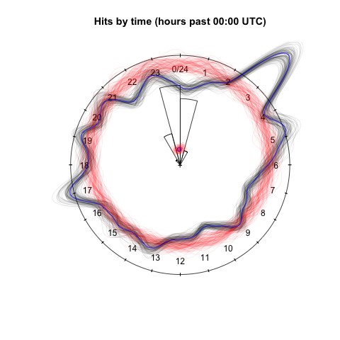
Visualization of bootstrap confidence procedures for maximum likelihood fit of von Mises distribution to time of day data.

The preceding analysis can be criticized as insufficiently skeptical. What if by some accident of chance, the observed data are unusually poorly- (or well-)fit by the model? What if model is inappropriate so that the theoretical standard errors don’t capture the actual uncertainty in the fit? A useful tool to address questions like these is the bootstrap, which relies on creating synthetic data through resampling (with replacement) of the real data itself rather than through its distillation into the fit model.

In the above figure, a smoothed version is given for each bootstrap resample of the data in a pale blue. These bands closely follow the original, almost obscuring it with their presence. The red loops are here fit to the same bootstrap resamples of the data, without a visually obvious difference. This is reassuring!

The wedges are a (radial) histogram for the distribution of \(\mu^*\) from the bootstrap resamples. In numbers, the bootstrap 95% confidence interval is [22:31 UTC, 00:55 UTC], much wider than the [23:29 UTC, 00:05 UTC] 95% confidence interval implicit in the theoretical standard errors. Finally, the blue dot and red cloud of dots near the center are the respective real data and bootstrap data values of the sample mean of the position \(z\). The inference procedure depends on the data directly through this value and it is again reassuring to see that it does not vary wildly under bootstrap resamples.

So this is most of the story for about the simplest model that can in good faith be applied to this data. Visualization, numerical results, and domain knowledge suggest a substantial mismatch between model and data. The problem seems to lie not in fitting but in formulation. In the final post in this series, I’ll take a look at a model that may do a better job of explaining this data by mixing over multiple von Mises distributions.