Pace pace mapping

If you don’t want to hear about code, just scroll down until you see an image!

Matplotlib’s hexbin functionality is remarkable, even by the standards of other hexagonal binning packages such as the hexbin package for R. To see why, we can take a look into the function’s (judiciously trimmed) docstring:

Make a hexagonal binning plot.

Call signature::

   hexbin(x, y, C = None, [...]
          reduce_C_function = np.mean, [...])

Make a hexagonal binning plot of *x* versus *y*, where *x*,
*y* are 1-D sequences of the same length, *N*. If *C* is *None*
(the default), this is a histogram of the number of occurences
of the observations at (x[i],y[i]).

If *C* is specified, it specifies values at the coordinate
(x[i],y[i]). These values are accumulated for each hexagonal
bin and then reduced according to *reduce_C_function*, which
defaults to numpy's mean function (np.mean).

Let’s unpack this in the context of the running visualization I’ve been experimenting with. My raw data is a collection of GPS tracks for my runs, which themselves are a sequence of latitude-longitude coordinates paired with times. With a little processing, these can be coordinates paired with duration spent around that location. The longitude, latitude, and duration are the respective x, y, and C.

The reduce_C_function is just a way of turning a list of values into a number.¹ For the visualization that shows the total time spent in each region, I can use the np.sum function, which adds up all the durations that have been accumulated into the bin.

(Exercise to the reader: if hexbin didn’t accept C = None, what C and reduce_C_function could you use to recover ordinary histogram behavior?)

(Exercise to the reader and myself: is there any situation in which the default reduce_C_function = np.mean is actually a reasonable choice?)

This is much more generality than I tend to associate with constructing a histogram, but it makes a lot of sense to think about it that way.² Or at least it pulls apart the two distinct sub-tasks of mapping a point to a bin and then doing something with that point and that bin. Here’s an example of something I can do with that extra generality:

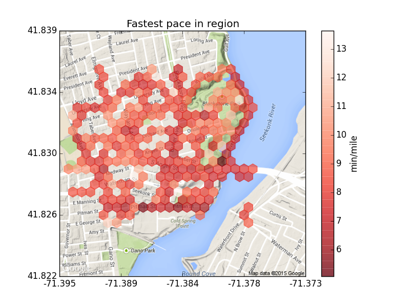
Wayland Square runs. Binning to 28×28 hexes.

Rather than pairing duration with locations, I pair my pace at the location.³ Then, rather than adding up the values in each region, I take the minimum (fastest) of the paces there to determine its color. It’s darker red where I’m going faster. The darkest red region at the acute angle made by Seekonk River and the Henderson Bridge is probably an artifact; going under the overpass may cause the GPS to behave unreliably.

Overall, the visualization is interesting but the data are too limited to say very much yet. I seem be able to go fastest along Pitman Street, which has the triple distinction of being a straightaway, at a very gentle slope, and at the beginning/end of many of my runs. I’m slowest in the curving trails of Blackstone Park.

It’s probably worth going through the menagerie of standard visualizations and seeing where else a count can be replaced with a more generic reduction.