Miss America BMI

(H/t to @roreiy for bringing this to my attention.)

The following provocative figure, taken from a page on “The Ideal Body Image and BMI”, has gone mildly viral recently:

Credit for this image goes to PsychGuides.com, who have requested that I “link back to the original source, which allows readers to learn more about the additional research as well as the methodology used for this project”.

Without going into the rhetoric or argument of the figure, I thought it was worth quickly replicating it from the available data to clear up some ambiguities. This should also save effort for anyone who wants to take a deeper dive into the subject.

I’m using a Miss America height/weight data set that was prepared, or at least made available, by Todd Swanson. The source for this data is from the accompanying website for the American Experience documentary about the pageant.

socket <- url("http://www.math.hope.edu/swanson/data/miss_america.txt")
ma.dat <- read.table(socket, skip=5, header=TRUE, na.strings=c("*"))
ma.dat[ma.dat$year > 1991,]

##    year                  name state age height weight
## 65 1992          Carolyn_Sapp    HI  24     70     NA
## 66 1993        Leanza_Cornett    FL  21     NA     NA
## 67 1994        Kimberly_Aiken    SC  18     NA     NA
## 68 1995    Heather_Whitestone    AL  21     NA     NA
## 69 1996        Shawntel_Smith    OK  24     NA     NA
## 70 1997     Tara_Dawn_Holland    KS  23     NA     NA
## 71 1998          Kate_Shindle    IL  21     71    145
## 72 1999        Nicole_Johnson    VA  24     69    133
## 73 2000  Heather_Renee_French    KY  24     66     NA
## 74 2001 Angela_Perez_Baraquio    HI  24     64    118
## 75 2002          Katie_Harman    OR  21     63    110

I print those post-1991 entries because they don’t show up in the PsychGuides.com figure. There is a note about this:

The average height and weight of winners was sporadically available up until 2002. Using the height and weights that were available, we were able to calculate BMIs for each winner.

However, the data is available for the 1998, 1999, 2001, and 2002 winners. One possibility is that whatever software they were using choked on the first */NA it encountered.

Moving on, I apply the standard BMI formula for height in inches and weight in pounds.

ma.dat$bmi <- ma.dat$weight / (ma.dat$height ** 2) * 703

Another methodology note mentions that “information on the average woman for each set of years was available through the Centers for Disease Control (CDC)”. Tracking this down required looking into three separate reports.¹ In all cases, “average” is taken to be the mean.² Also, in all cases, we’ll be looking just at data for US women aged 20–29.

From Table 10 in CDC report “Mean Body Weight, Height, and Body Mass Index, United States 1960–2002”, we have:

us.year <- c(1960:1962,1971:1974,1976:1980,1988:1994,1999:2002)
us.bmi <- c(rep(22.2,3),rep(23.0,4),rep(23.1,5),rep(24.3,7),rep(26.8,4))

From Table 14 in CDC report “Anthropometric Reference Data for Children and Adults: United States, 2003–2006”, we have

us.year <- c(us.year,2003:2006)
us.bmi <- c(us.bmi,rep(26.5,4))

Unlike the first report, this one also contains quantiles for BMI. As a quick summary, for 2003–2006, the (10%, 50%, 90%) quantiles are (19.4, 24.4, 35.9).

Finally, from Table 14 in CDC report “Anthropometric Reference Data for Children and Adults: United States, 2007–2010”, we have:

us.year <- c(us.year,2007:2010)
us.bmi <- c(us.bmi,rep(27.5,4))

For 2007–2010, the (10%, 50%, 90%) quantiles are (19.9, 25.3, 38.0).

Out of caution and pedantry, when I assemble all of these observations into a data frame, I reweight them to compensate for the difference of lengths in the periods covered. Even though it is visually helpful to see three separate points for, e.g., 1960, 1961, and 1962, the code computing a linear trend should not treat them as (unusually consistent) independent observations.

us.dat <- data.frame(year=us.year, bmi=us.bmi)
us.dat$weight <- c(rep(1/3,3),rep(1/4,4),rep(1/5,5),rep(1/7,7),rep(1/4,4),rep(1/4,4),rep(1/4,4))

With all the preliminary work done, the two data sets can be plotted using a slightly inelegant invocation of ggplot2.

require(ggplot2)

## Loading required package: ggplot2

ggplot(us.dat, aes(x=year,y=bmi,weight=weight)) +
  geom_point(color="skyblue") +
  geom_smooth(method="lm",fullrange=TRUE) +
  geom_point(data=ma.dat, aes(x=year,y=bmi), color = "navy") +
  geom_smooth(data=ma.dat, aes(x=year,y=bmi), method="loess") +
  xlab("Year") +
  ylab("BMI")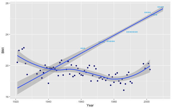

BMI Trends: The Average American Woman vs. Miss America

There’s really no good reason to fit a linear trend to the Miss America data, especially given the new observations, so I instead use LOESS. There’s really, really no good reason to fit a linear trend to the American average data, so I leave that choice intact.