Noise level and imbalance

In a paper called Learning without Concentration (which for the life of me, I have no idea how I ended up reading), I came across the concept of “noise level”. It probably has another name—it’s a fairly natural idea but searching under that name don’t turn up much of relevance—but I have no idea what that is. In any case, it names the minimum expected loss of a predictor for a particular joint distribution of predictor and outcome taken over some class of functions. In the case when the loss function is squared-error (\(L_2\) norm), it could roughly be called minimum mean integrated squared error.

I’ve been investigating a certain class of infinitely imbalanced logistic regression models. Suppose that we have independent predictors \[X_1, \ldots, X_n \sim \text{Normal}(0,1)\] and independent outcomes \[Y_i | (X_i = x) \sim \text{Bernoulli}(\text{logit}^{-1}(\theta \sigma_n X_n + \kappa_n)).\] The \(\sigma_n\) term determines how the effect term \(\theta\) is scaled based on the number of observations when the offset term \(\kappa_n\)¹ is such that the expected number of positive outcomes (\(\sum_{i=1,\ldots,n} \mathbb{E}[Y_i]\)) is \(\lambda\).

In this framework,² the noise level is \[ ||f^* - Y||_{L_2} := \min_{\theta, \lambda} (\mathbb{E}[(Y_1 - \text{logit}^{-1}(\theta \sigma_n X_1 + \kappa_n(\lambda)))^2])^{1/2}. \] I haven’t attempted to evaluate the expectation analytically, but it can be approximated by Monte Carlo. Then a minimizer that is suitably robust to a stochastic objective function can be used to take the minimum with respect to \(\theta\) and \(\lambda\).

I did a little numerical experiment and the results are a bit surprising. As a final piece of setup, I define \[ ||f - Y||_{L_2} := \mathbb{E}[(Y_1 - \text{logit}^{-1}(\theta \sigma_n X_1 + \kappa_n(\lambda)))^2])^{1/2}, \] that is, the mean integrated squared error under the model that generated the data. We might call this the “noise at truth”.

(Exercise for the reader: can we say anything about which of \(||f^* - Y||_{L_2}\) and \(||f - Y||_{L_2}\) is larger?)

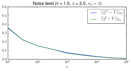
Constant effect term rescaling.

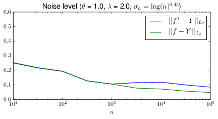
Slowly-growing effect term rescaling.

Without the effect term rescaling, the noise level quickly tends towards zero. From the connotations of noise level, this sounds like a great thing! But examination of \(\lambda_{\text{opt}}\) shows that it is tending to zero, away from its true value. The intution is that a predictor that makes the probability of a positive outcome go to zero everywhere will incur, on average, a large loss on \(\lambda\) observations and a small loss on \(n - \lambda\) observations. This may be acceptable for prediction but it fouls things up if it’s important to learn the effect term \(\theta\). A slowly-growing effect term rescaling can prevent this failure mode (and I’m currently writing up the details of how this works). Paradoxically, the scaling helps by raising the noise level, thereby making prediction harder!

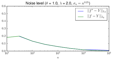
This “slowly-” part also turns out to be critical. When I switch from sedate \(o(\log(n)^{0.5})\) growth to a galloping \(\Theta(n^{0.25})\), the rapid decrease in the noise level returns.

“Rapid” effect term rescaling.