Sparse conditional inference
Quick proof-of-concept post just to test out my knitr/hakyll workflow.
Working as a Bayesian, all the analysis you do is conditional. In particular, you condition on the observed data and, more philosophically, on the your priors, hyperpriors, model structure, etc. As a frequentist, you have more freedom about what aspects of experimental setup or outcomes you condition on. A 1995 paper by Nancy Reid, “The Roles of Conditioning in Inference”, reviews the situation and sketches how standard inferential procedures can be adapted into conditional ones.
While this adaptation cannot be done automatically in general, Alessandra Brazzale handled the case of logistic and loglinear modes, and implemented the procedure in the R package cond. The hoa vignette demonstrates its usage, along with that of the related marg and nlreg packages.
I’m going to run a quick example of how this package can be used for the analysis of array-structured data, and what happens when the outcome is heavily imbalanced. When the array is interpreted as the adjacency matrix of a network and the imbalance is towards negative outcomes, i.e., the absence of edges, it seems more appropriate to describe the imbalance as sparsity.
For a data model, suppose that we have independent \(Y_{ij} \sim \text{Bernoulli}(\text{logit}^{-1}(\theta X_{ij} + \alpha_i + \beta_j + \kappa))\), arranged by respective rows and columns \(1 \leq i, j \leq d\), for a total of \(n = d^2\) observations. We can whip up a function to generate data from this model, supposing that covariates \(X_{ij}\), row effects \(\alpha_i\), and column effects \(\beta_i\) are all drawn as independent unit normals.
make.data <- function(d, theta, kappa) {
	n <- d ** 2

	dat <- data.frame(matrix(nrow = n, ncol = 3))
	colnames(dat) <- c("row", "col", "logit.p")
	dat$row <- 1:d
	dat$col <- sort(dat$row)

	dat$x <- rnorm(n, 0, 1)

	alpha <- rnorm(d, 0, 1)
	beta  <- rnorm(d, 0, 1)

	for(i in 1:n) {
		dat$logit.p[i] <- theta * dat$x[i] +
		alpha[dat$row[i]] + beta[dat$col[i]] + kappa
	}

	dat$p <- exp(dat$logit.p) / (1 + exp(dat$logit.p))

	dat$y <- runif(n) < dat$p

	dat$row <- factor(dat$row)
	dat$col <- factor(dat$col)
	dat
}
We generate two realization of this model: a dense case and a sparse case.
d <- 15
theta <- 0.5
d.dense <- make.data(d, theta, kappa = 0.0)
d.sparse <- make.data(d, theta, kappa = -3.5)
We can see the difference between the two cases by, for example, comparing their row sums.
aggregate(y ~ row, data = d.dense, sum)## row y
## 1 1 9
## 2 2 10
## 3 3 13
## 4 4 5
## 5 5 7
## 6 6 7
## 7 7 10
## 8 8 11
## 9 9 7
## 10 10 13
## 11 11 9
## 12 12 9
## 13 13 0
## 14 14 4
## 15 15 13aggregate(y ~ row, data = d.sparse, sum)## row y
## 1 1 0
## 2 2 2
## 3 3 0
## 4 4 0
## 5 5 0
## 6 6 1
## 7 7 1
## 8 8 0
## 9 9 3
## 10 10 2
## 11 11 0
## 12 12 1
## 13 13 0
## 14 14 3
## 15 15 1Row and column sums of 0 (and likewise of \(d\), though we don’t encounter any here) are a problem for inference since they send MLE for the corresponding effects towards negative infinity (respectively, positive infinity). If we’re interested only in \(\theta\), and let’s suppose we are, such rows and column can safely be dropped from the data and the model.
glm.zeros <- function(data) {
	rs <- aggregate(y ~ row, data=data, sum)
	cs <- aggregate(y ~ col, data=data, sum)

	rnz <- rs$row[rs$y != 0]
	cnz <- cs$col[cs$y != 0]

	dnz <- data[data$row %in% rnz,]
	dnz <- dnz[dnz$col %in% cnz,]

	list(fm=glm(y ~ x + C(row, how.many=length(rnz)-2) + C(col,
	how.many=length(cnz)-2), family=binomial("logit"), data=dnz), dnz=dnz)
}
Using this procedure, we can get point estimates for \(\kappa\) and \(\theta\) (denoted as (Intercept) and x in output below). Point estimates for the length(rnz)-2 identifiable row effects and length(cnz)-2 identifiable column effects
fm.dense <- glm.zeros(d.dense)## Warning: contrasts dropped from factor C(row, how.many =
## length(rnz) - 2) due to missing levelsfm.dense$fm$coef[1:2]## (Intercept) x
## 0.9969 0.6816fm.sparse <- glm.zeros(d.sparse)## Warning: contrasts dropped from factor C(row, how.many =
## length(rnz) - 2) due to missing levels## Warning: contrasts dropped from factor C(col, how.many =
## length(cnz) - 2) due to missing levelsfm.sparse$fm$coef[1:2]## (Intercept) x
## -2.818 1.056In the dense case, the estimate for \(\theta\) is not too bad (recall that the true value of \(\theta\), from which the data was generated, is 0.5). In the sparse case, the sign of the estimate for \(\theta\) is correct but the magnitude is way off. Is there a way to improve this?
The idea of conditional inference, in this case, is to treat the observed row and column sums as an immutable part of the data generating process. Consequently, we consider realization where the total sum of positive outcomes is fixed. Since this sum is a sufficient statistic for \(\kappa\), the conditional model will not be informative about \(\kappa\). This is desirable, since \(\kappa\) is no longer meaningful in this model after we have removed rows and columns in a data-dependent way. In addition to any of its other benefits, conditioning has allowed us to side-step model misspecification.
require(cond)## Loading required package: cond## Loading required package: statmod## Loading required package: survival##
## Package "cond" 1.2-3 (2014-06-27)
## Copyright (C) 2000-2014 A. R. Brazzale
##
## This is free software, and you are welcome to redistribute
## it and/or modify it under the terms of the GNU General
## Public License published by the Free Software Foundation.
## Package "cond" comes with ABSOLUTELY NO WARRANTY.
##
## type `help(package="cond")' for summary informationdnz <- fm.sparse$dnz
cm.sparse <- cond(fm.sparse$fm, offset=x)
coef(cm.sparse)## Estimate Std. Error
## uncond. 1.0560 0.4636
## cond. 0.7458 0.3687In this particular case, the conditional MLE produces a better point estimate than the profile MLE.
plot.cond(cm.sparse, which=2)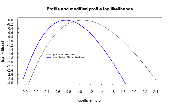
Comparison of log-likelihood for modified profile likelihood (conditional) and profile likelihood (unconditional) on sparse arrary synthetic data.